Deconvolution with scaden for spatial transcriptomics data

Compiled: April 12, 2023

Recent studies (Zubair el.al., Wang el.al.) have indicated the potential to apply bulk-deconvolution methods to new technologies such as spatial transcriptomics when the resolution is not at single-cell level.

For this tutorial, we will use scaden to deconvolute a dataset of sagital mouse brain slices generated using the Visium v1 chemistry, and generate cell-type specific gene expression. The data is provided by Seurat package and can be downloaded via InstallData(). If you haven’t installed scaden, please follow instruction here.

Load required libraries and data

## download data if it's not already installed
SeuratData::InstallData("stxBrain")

library(SCdeconR)
library(plotly)
## load brain spatial data from sample anterior1
brain <- SeuratData::LoadData("stxBrain", type = "anterior1")
## proprocess data
brain <- SCTransform(brain, assay = "Spatial", verbose = FALSE)
## see ?refdata_brain for details
data("refdata_brain")

Perform spot deconvolution using scaden

## provide directory that contains python binary to pythonpath, e.g. /usr/bin/
decon_res <- scdecon(bulk = GetAssayData(brain, slot = "data", assay = "SCT"), ref = GetAssayData(refdata_brain,
    slot = "data", assay = "SCT"), phenodata = refdata_brain@meta.data, filter_ref = TRUE, decon_method = "scaden",
    norm_method = "none", trans_method = "none", marker_strategy = "all", pythonpath = "/path/to/python/bin/dir/",
    tmpdir = "/path/to/tmp/dir/")

Visualize distribution of cell-type proprotions

prop_barplot(prop = decon_res[[1]], interactive = TRUE)

Add predicted cell-type proportions as new assaydata to Seurat object.

prop_assay <- CreateAssayObject(data = decon_res[[1]])
brain[["PROP"]] <- prop_assay

Visualize predicted cell proportions for L5 IT, L6 IT and macrophage in spatial

DefaultAssay(brain) <- "PROP"
SpatialFeaturePlot(brain, features = c("L5.IT", "L6.IT"), pt.size.factor = 1.6, ncol = 2)

Compute cell-type specific gene expression

ct_exprs_list <- celltype_expression(bulk = GetAssayData(brain, slot = "data", assay = "SCT"), ref = GetAssayData(refdata_brain,
    slot = "data", assay = "SCT"), phenodata = refdata_brain@meta.data, prop = decon_res[[1]], UMI_min = 0,
    CELL_MIN_INSTANCE = 1)

## 
##      Astro       Endo    L2.3.IT         L4      L5.IT      L5.PT      L6.CT 
##         20         20         20         20         20         20         20 
##      L6.IT        L6b      Lamp5 Macrophage      Meis2         NP      Oligo 
##         20         20         20         20         20         20         20 
##       Peri      Pvalb        SMC   Serpinf1       Sncg        Sst       VLMC 
##         20         20         20         20         20         20         20 
##        Vip 
##         20

## create assaydata and add to Seurat object
for (i in 1:length(ct_exprs_list)) {
    ct_assay <- CreateAssayObject(data = as.matrix(ct_exprs_list[[i]]))
    ct_name <- names(ct_exprs_list)[i]
    brain[[ct_name]] <- ct_assay
}

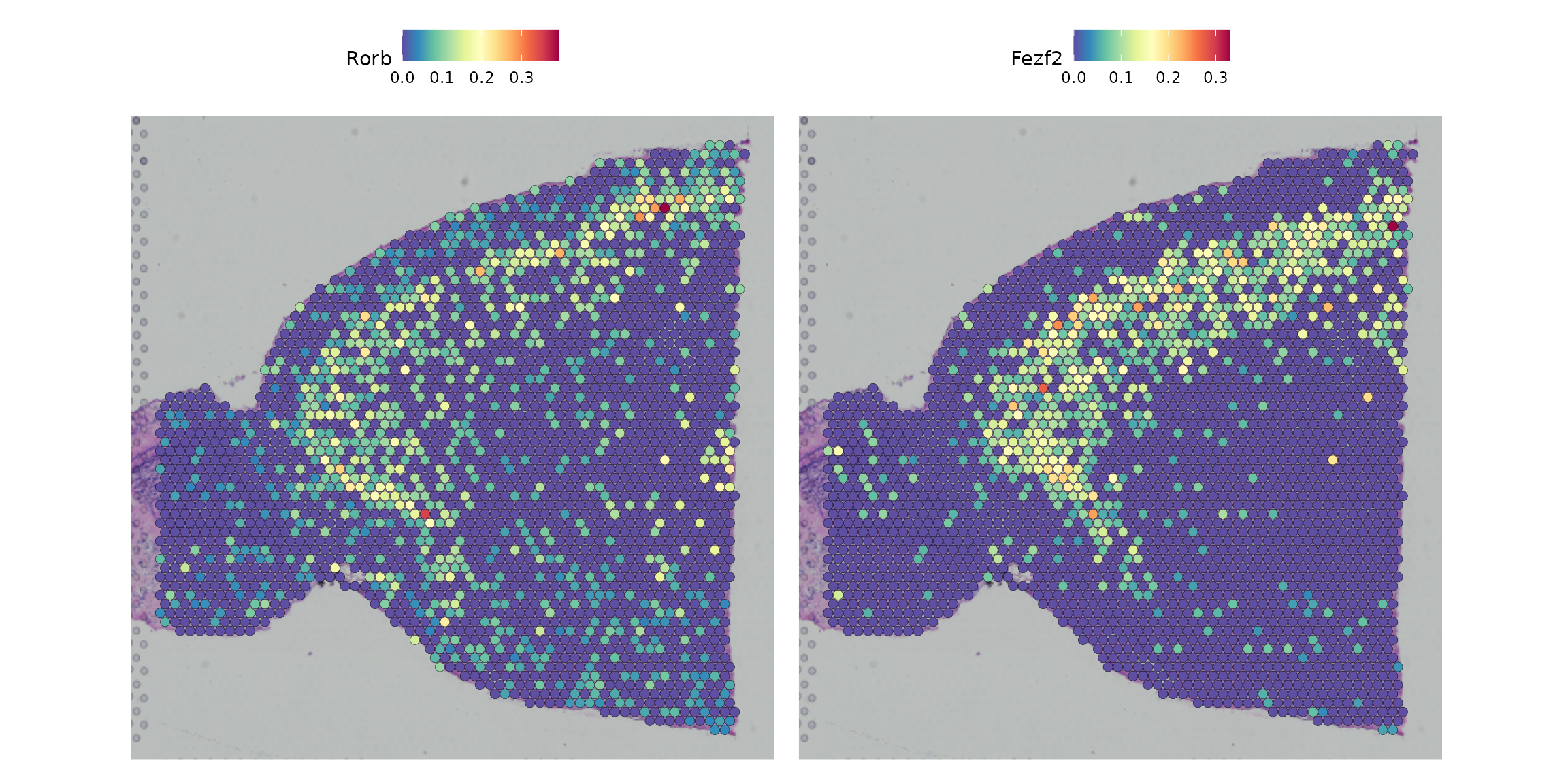
We can then examine expression of genes using cell-type specific gene expression assays

DefaultAssay(brain) <- "L5.IT"
SpatialFeaturePlot(brain, features = c("Rorb", "Fezf2"), pt.size.factor = 1.6, ncol = 2)